Transforming data

Motivation

Data rarely comes in the form we need it in, hence we need to transform it.

In this lesson we’ll transform data using another tidyverse package dplyr to:

• change the focus. For example, filtering data for (observations) rows or selecting (variables) columns of interest.
• create new variables that are functions of existing variables. For example, transforming separate day, month and year variables into a single data variable.
• calculate summarised data such as observations per three months.

Often these operations can be combined, known as piping, which is very powerful and convenient.

Our goal is to reproduce the analysis of the 1994 Heske et. al. paper is that there is evidence that kangaroo rats compete directly with four other rodent species, generating a similar figure to the one below, to confirm their observations.

Concretely, we are going to look at the effect of kangaroo rat exclusion on the populations of smaller granivores in two 0.25 hectare plots versus two plots where kangaroo rats were allowed access.

Panels A and B shows the number of captures of threes species of kangaroo rats and five species of smaller granivore rodents over a period from 1977 to 1990. Panel A shows the populations when the eight species were left to compete for resources and Panel B shows the effect of excluding the kangaroo Rats.

For simplicity we’re going to ignore Panel C, which examines grasshopper rats, and only

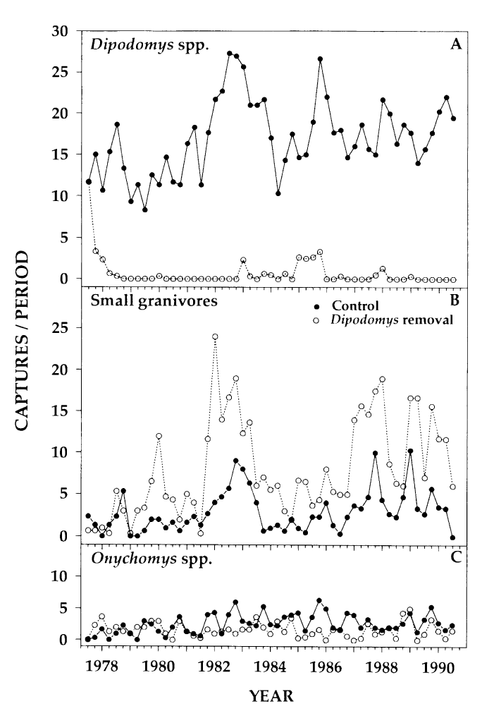
Figure 1 from Heske et. al., 1994

Filtering observations

The first verb to consider is filter which enables us to subset observations based on their value.

Consider the surveys data and sub-setting observations that only occurred from 1985 onwards. It’s fairly natural to say “filter the survey where the year variable is equal or greater than 1985”. And indeed this is how we use filter as a verb.

In the code below, we give the filter function two arguments. The first is the data frame, the second is the variable and condition on which we wish to filter.

(Note that we aren’t assigning the output to an object here, so we can see it.)

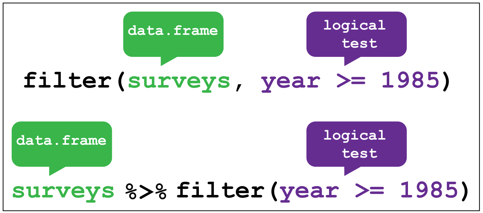
# Filter observations that only occurred from 1985 onwards
 filter(surveys, year >= 1985)

#> # A tibble: 25,290 × 13
#>    record_id month   day  year plot_id species_id   sex hindfoot_length
#>        <int> <int> <int> <int>   <int>      <chr> <chr>           <int>
#> 1      10606     7    24  1985       2         NL     F              30
#> 2      10617     7    24  1985       2         NL     M              32
#> 3      10627     7    24  1985       2         NL     F              32
#> 4      10720     8    20  1985       2         NL     F              31
#> 5      10923    10    13  1985       2         NL     F              31
#> 6      10949    10    13  1985       2         NL     F              33
#> 7      11215    12     8  1985       2         NL     F              32
#> 8      11329     3     9  1986       2         NL     M              34
#> 9      11496     5    11  1986       2         NL     F              31
#> 10     11498     5    11  1986       2         NL     F              31
#> # ... with 25,280 more rows, and 5 more variables: weight <int>,
#> #   genus <chr>, species <chr>, taxa <chr>, plot_type <chr>

We could even do this for a specific date and species (assuming we know there was an observation), using values for day, month, year and species.

# Filter observations that only occurred on the 9th of March 1986
 filter(surveys, month == 3, day == 9, year == 1986, species_id == "NL")

#> # A tibble: 2 × 13
#>   record_id month   day  year plot_id species_id   sex hindfoot_length
#>       <int> <int> <int> <int>   <int>      <chr> <chr>           <int>
#> 1     11329     3     9  1986       2         NL     M              34
#> 2     11302     3     9  1986       3         NL     F              30
#> # ... with 5 more variables: weight <int>, genus <chr>, species <chr>,
#> #   taxa <chr>, plot_type <chr>

An alternative way to use filter is to “pipe” the function using %>% which you can think of as using the word “then”. We take our data set then filter it.

This makes more sense when combining several operations, but even with one operation it means we only have to provide the values argument to the filter, like so:

# Pipe the filter for observations that only occurred on the 9th of March 1986
surveys %>% filter(month == 3, day == 9, year == 1986, species_id == "NL")

#> # A tibble: 2 × 13
#>   record_id month   day  year plot_id species_id   sex hindfoot_length
#>       <int> <int> <int> <int>   <int>      <chr> <chr>           <int>
#> 1     11329     3     9  1986       2         NL     M              34
#> 2     11302     3     9  1986       3         NL     F              30
#> # ... with 5 more variables: weight <int>, genus <chr>, species <chr>,
#> #   taxa <chr>, plot_type <chr>

Armed with this information, let’s filter the data for the period covered in the paper figure, from the start of the surveys in 1977 until the end of 1990.

Challenge

Filter the surveys from 1977 until 1990 and assign the output to surveys_filtered

Using the pipe %>% is optional, but recommended.

Ctl+Shift+M is a shortcut to create a pipe.

See SQL basic queries lesson to compare using dplyr in R with filtering and selecting in SQL.

To reproduce the analysis in the paper we need to know which which four plots the different treatments were carried out on.

The codes for the twenty four plots are found here.

To save time, here is a summary of the ones we need, which you can paste into your script:

# Control Plots: 2,8,12,22
# Treatment Plots: 3,15,19,21

# Create a vector for the experimental plots
exp_plots <- c(8,11,12,14,3,15,19,21)

# Keep only the rows corresponding with the experimental plot_id's
surveys_filtered <- surveys_filtered %>% filter(plot_id %in% exp_plots)

Arranging observations

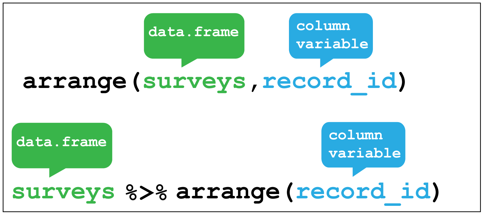
Although we don’t need to do this here, it is worth mentioning the other key verb for working with the observations in the rows is arrange() which enables you to arrange the observations in a data frame according to one or more variables.

As with filter() we supply the variable or variables of interest as the arguments to arrange().

For example we could arrange the observations according to the record_id variable:

# Look at the original order of the observations
surveys

#> # A tibble: 34,786 × 13
#>    record_id month   day  year plot_id species_id   sex hindfoot_length
#>        <int> <int> <int> <int>   <int>      <chr> <chr>           <int>
#> 1          1     7    16  1977       2         NL     M              32
#> 2         72     8    19  1977       2         NL     M              31
#> 3        224     9    13  1977       2         NL  <NA>              NA
#> 4        266    10    16  1977       2         NL  <NA>              NA
#> 5        349    11    12  1977       2         NL  <NA>              NA
#> 6        363    11    12  1977       2         NL  <NA>              NA
#> 7        435    12    10  1977       2         NL  <NA>              NA
#> 8        506     1     8  1978       2         NL  <NA>              NA
#> 9        588     2    18  1978       2         NL     M              NA
#> 10       661     3    11  1978       2         NL  <NA>              NA
#> # ... with 34,776 more rows, and 5 more variables: weight <int>,
#> #   genus <chr>, species <chr>, taxa <chr>, plot_type <chr>

# Arrange the surveys according to record_id. Note the default is ascending order
surveys %>% arrange(record_id)

#> # A tibble: 34,786 × 13
#>    record_id month   day  year plot_id species_id   sex hindfoot_length
#>        <int> <int> <int> <int>   <int>      <chr> <chr>           <int>
#> 1          1     7    16  1977       2         NL     M              32
#> 2          2     7    16  1977       3         NL     M              33
#> 3          3     7    16  1977       2         DM     F              37
#> 4          4     7    16  1977       7         DM     M              36
#> 5          5     7    16  1977       3         DM     M              35
#> 6          6     7    16  1977       1         PF     M              14
#> 7          7     7    16  1977       2         PE     F              NA
#> 8          8     7    16  1977       1         DM     M              37
#> 9          9     7    16  1977       1         DM     F              34
#> 10        10     7    16  1977       6         PF     F              20
#> # ... with 34,776 more rows, and 5 more variables: weight <int>,
#> #   genus <chr>, species <chr>, taxa <chr>, plot_type <chr>

Check out the ?arrange for more examples and information about using this function.

Selecting variables

Selecting the variables contained in the columns can be done in various ways. For example, by the column number, the variable name or by range. Check the help function ?select for more options.

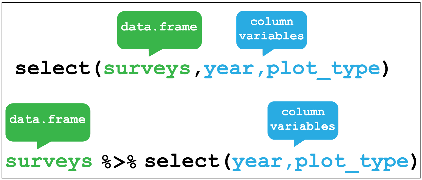
# Select the year and plot type columns
surveys %>% select(year,plot_type)

#> # A tibble: 34,786 × 2
#>     year plot_type
#>    <int>     <chr>
#> 1   1977   Control
#> 2   1977   Control
#> 3   1977   Control
#> 4   1977   Control
#> 5   1977   Control
#> 6   1977   Control
#> 7   1977   Control
#> 8   1978   Control
#> 9   1978   Control
#> 10  1978   Control
#> # ... with 34,776 more rows

As we saw earlier, we have thirteen variables in the surveys data, but we don’t need all of them. Specifically we don’t need the sex, the hind-foot length or the weight of the animals. We’re just interested in the population changes over time.

Rather than selecting the columns we want, an alternative is to drop the ones we don’t using a minus sign in front of the variable name, like so:

# Select everything except sex, hindfoot and weight
surveys_selected <- surveys_filtered %>% select(-sex,-hindfoot_length,-weight)

# Check the output
glimpse(surveys_selected)

#> Observations: 6,236
#> Variables: 10
#> $ record_id  <int> 2, 344, 509, 655, 755, 886, 1083, 1087, 1250, 1361,...
#> $ month      <int> 7, 10, 1, 3, 4, 5, 7, 7, 9, 10, 6, 8, 10, 11, 1, 2,...
#> $ day        <int> 16, 18, 8, 11, 8, 18, 8, 8, 4, 8, 23, 14, 26, 23, 1...
#> $ year       <int> 1977, 1977, 1978, 1978, 1978, 1978, 1978, 1978, 197...
#> $ plot_id    <int> 3, 3, 3, 3, 3, 3, 3, 3, 3, 3, 3, 3, 3, 3, 3, 3, 3, ...
#> $ species_id <chr> "NL", "NL", "NL", "NL", "NL", "NL", "NL", "NL", "NL...
#> $ genus      <chr> "Neotoma", "Neotoma", "Neotoma", "Neotoma", "Neotom...
#> $ species    <chr> "albigula", "albigula", "albigula", "albigula", "al...
#> $ taxa       <chr> "Rodent", "Rodent", "Rodent", "Rodent", "Rodent", "...
#> $ plot_type  <chr> "Long-term Krat Exclosure", "Long-term Krat Exclosu...

Creating new variables

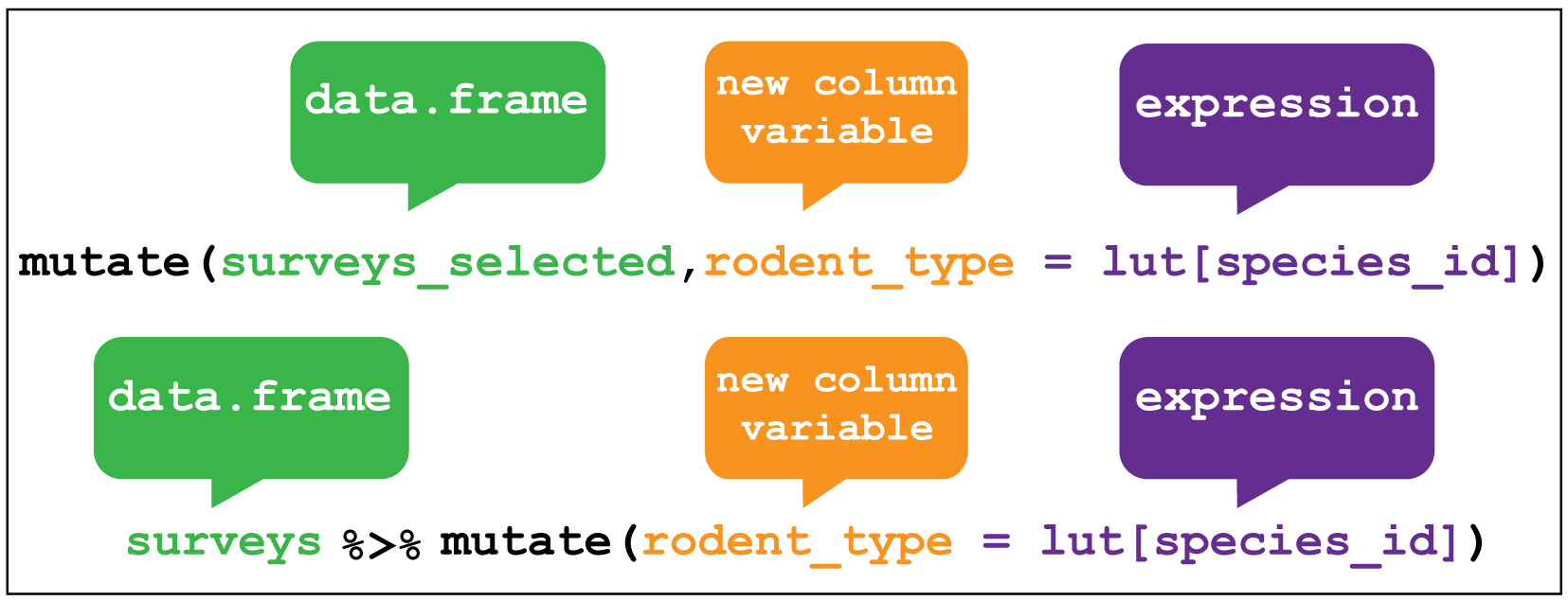
Often we need to create new variables that are functions of existing columns. For example, in the survey data there are forty species, of which we are only interested in eight. Moreover, we are interested in comparing the three Kangaroo Rat species with the five smaller granivores, so it would be useful to have a variable the categorised the rodents as either “Kangaroo Rat” or “Carnivore”.

We could do this using mutate to create a rodent_type variable that is a function of the species_id column.

This is a little tricky, but the steps are as follows:

1. We create a lookup table in the form of a named vector which we’ll call lut. The names of each element in lut correspond with one of the eight species_id we are interested in.. The values of each named element are either Kangaroo Rat or Granivore.

2. Next we can use the lookup table to filter surveys_selected for observations where the species_id match the names of the lookup table elements by passing lut as an argument to the function names().

3. Now when we subset the lookup table with a character string, here species_id from the surveys_selected, it will return the values in the lookup table that correspond with the names in the species_id character string. For example, subsetting "DM" in the lookup table will return the value Kangaroo Rat.

4. Using mutate we can create a new variable called rodent_type that contains the values return from subsetting the lookup table using species_id from the surveys_selected.

The codes associated with the forty species in the survey data are found here, but to save time the relevant codes are shown below. These codes are used to createthe lookup table lut as shown.

# Kangeroo Rats:
# DM    Dipodomys merriami          Rodent  Merriam's kangaroo rat
# DO    Dipodomys ordii             Rodent  Ord's kangaroo rat
# DS    Dipodomys spectabilis       Rodent  Banner-tailed kangaroo rat

# Granivores:
# PP    Chaetodipus penicillatus    Rodent  Desert pocket mouse
# PF    Perognathus flavus          Rodent  Silky pocket mouse
# PE    Peromyscus eremicus         Rodent  Cactus mouse
# PM    Peromyscus maniculatus      Rodent  Deer Mouse
# RM    Reithrodontomys megalotis   Rodent  Western harvest mouse

# Create a named vector as a lookup table, where the names of each vector
# element correspond with the species_id, and the values of each vector 
# element are either Kangaroo Rat or Granivore
lut <- c("DM" = "Kangaroo Rat",
         "DO" = "Kangaroo Rat",
         "DS" = "Kangaroo Rat",
         "PP" = "Granivore",
         "PF" = "Granivore",
         "PE" = "Granivore",
         "PM" = "Granivore",
         "RM" = "Granivore")

# Mutate surveys_selected
surveys_mutate_rodent <- surveys_selected %>%
  # Filter for observations only for the eight rodents species.
  # The condition is where species_id matches the names of the lookup table
  # vector elements
  filter(species_id %in% names(lut)) %>% 
  # Create a new variable called rodent_type as a function of species_id
  # by using the look-up table to return values of Kangaroo Rat and Granivore
  # that match the species_id code.
  mutate(rodent_type = lut[species_id])

# Check the output using a summary pipe, we should have 8 species of 2 types
surveys_mutate_rodent %>% group_by(species_id,rodent_type) %>% summarise()

#> Source: local data frame [8 x 2]
#> Groups: species_id [?]
#> 
#>   species_id  rodent_type
#>        <chr>        <chr>
#> 1         DM Kangaroo Rat
#> 2         DO Kangaroo Rat
#> 3         DS Kangaroo Rat
#> 4         PE    Granivore
#> 5         PF    Granivore
#> 6         PM    Granivore
#> 7         PP    Granivore
#> 8         RM    Granivore

We’ll come back to group_by() and summarise() very shortly.

Secondly it would be much more convenient to have a single date variable, and we can make one as a function of the day,month and year variables using another tidyverse package called lubridate.

Don’t worry to much about the details of the code, it’s the concept that matters.

We call the lubridate function dmy() explicitly by using the package name followed by two colons. This in turn uses the sprintf() function to parse the column variables.

# Mutate surveys_selected to create a Date column from the day,month and year
# variables
surveys_mutate_date <- surveys_mutate_rodent %>%
  # Convert day, month and year using lubridate
  mutate(date = lubridate::dmy(sprintf('%02d%02d%04d', day, month, year)))

# Check the output
glimpse(surveys_mutate_date)

#> Observations: 4,795
#> Variables: 12
#> $ record_id   <int> 5, 13, 63, 221, 303, 315, 1279, 2341, 2462, 3013, ...
#> $ month       <int> 7, 7, 8, 9, 10, 10, 9, 1, 2, 5, 11, 11, 1, 1, 3, 3...
#> $ day         <int> 16, 16, 19, 13, 17, 17, 4, 16, 25, 25, 9, 9, 12, 1...
#> $ year        <int> 1977, 1977, 1977, 1977, 1977, 1977, 1978, 1980, 19...
#> $ plot_id     <int> 3, 3, 3, 3, 3, 3, 3, 3, 3, 3, 3, 3, 3, 3, 3, 3, 3,...
#> $ species_id  <chr> "DM", "DM", "DM", "DM", "DM", "DM", "DM", "DM", "D...
#> $ genus       <chr> "Dipodomys", "Dipodomys", "Dipodomys", "Dipodomys"...
#> $ species     <chr> "merriami", "merriami", "merriami", "merriami", "m...
#> $ taxa        <chr> "Rodent", "Rodent", "Rodent", "Rodent", "Rodent", ...
#> $ plot_type   <chr> "Long-term Krat Exclosure", "Long-term Krat Exclos...
#> $ rodent_type <chr> "Kangaroo Rat", "Kangaroo Rat", "Kangaroo Rat", "K...
#> $ date        <date> 1977-07-16, 1977-07-16, 1977-08-19, 1977-09-13, 1...

Challenge

Create a data frame called surveys_kg with a new variable that converts the the original data frame surveys weight variable to kilograms, call the new variable weight_kg.

weight is in grams, so you need to divide by 1000 to convert to kg. Missing values can be removed using the filter() and is.na() functions like so: filter(!is.na(weight)). We need ! to make it “is not a NA”.

See SQL basic queries lesson to compare using dplyr in R with performing calculations in SQL.

Putting it all together

Rather than doing each of these steps individually, we could pipe these four operations together to create our surveys_subset data frame.

Note here, we’ve added another variable called quarter which calculates the three monthly date period. This is what they plotted in the paper, which is then helpful for comparing our plot to the published one.

surveys_subset <- surveys %>% 
  # Filter observations from 1977 to 1990, for the 3 K-rats and 5 granivores, 
  # and for the 4 experimental plots
  filter(year <= 1990,                    
         species_id %in% names(lut),         
         plot_id %in% exp_plots) %>%      
  # Use lookup table to create variable to indicate whether species is K-rat 
  # or Granivore
  mutate(rodent_type = lut[species_id],
         # Make combined date variable
         date = lubridate::dmy(sprintf('%02d%02d%04d', 
                                       day, month, year)),
  # Add the quartley period
  quarter = lubridate::quarter(date,with_year = TRUE)) %>% 
  # Drop unwanted variables
  select(-sex,-hindfoot_length,-weight)

Grouped summaries

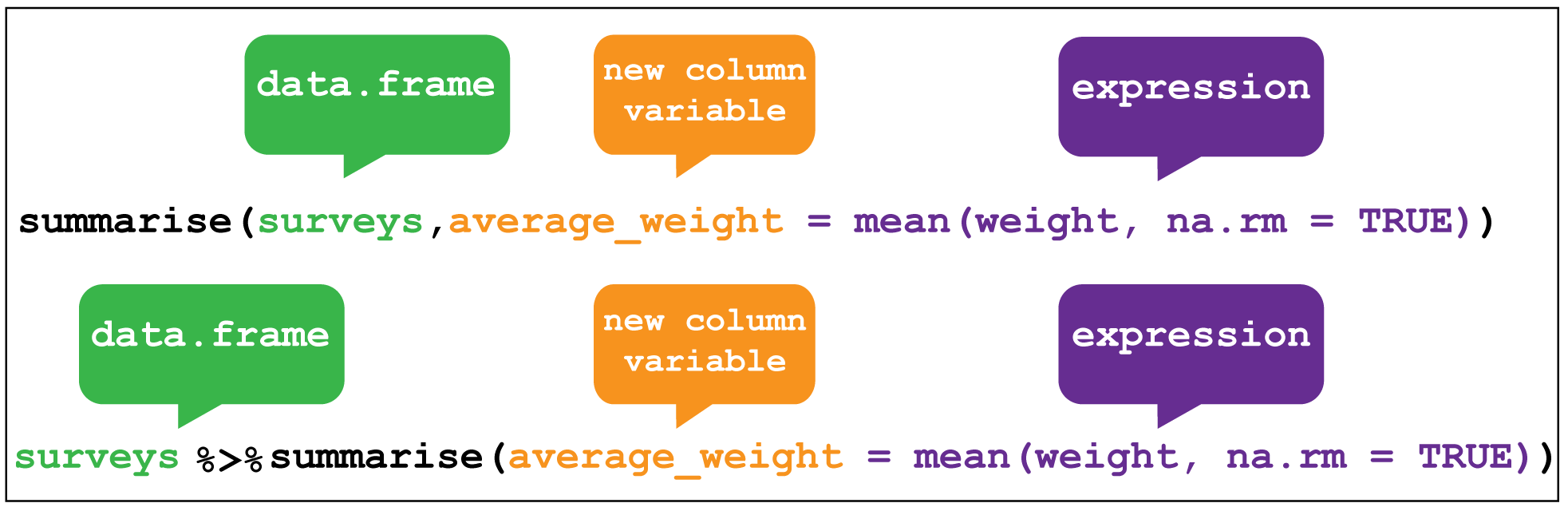
The last verb we’ll consider is summarise(), which collapses a data frame into a single row. For example, we could use it to find the average weight of all the animals surveyed in the original data frame using mean(). (Here the na.rm = TRUE argument is given to remove missing values from the data, otherwise R would return NA when trying to average.)

surveys %>% summarise(average_weight = mean(weight,na.rm=TRUE))

#> # A tibble: 1 × 1
#>   average_weight
#>            <dbl>
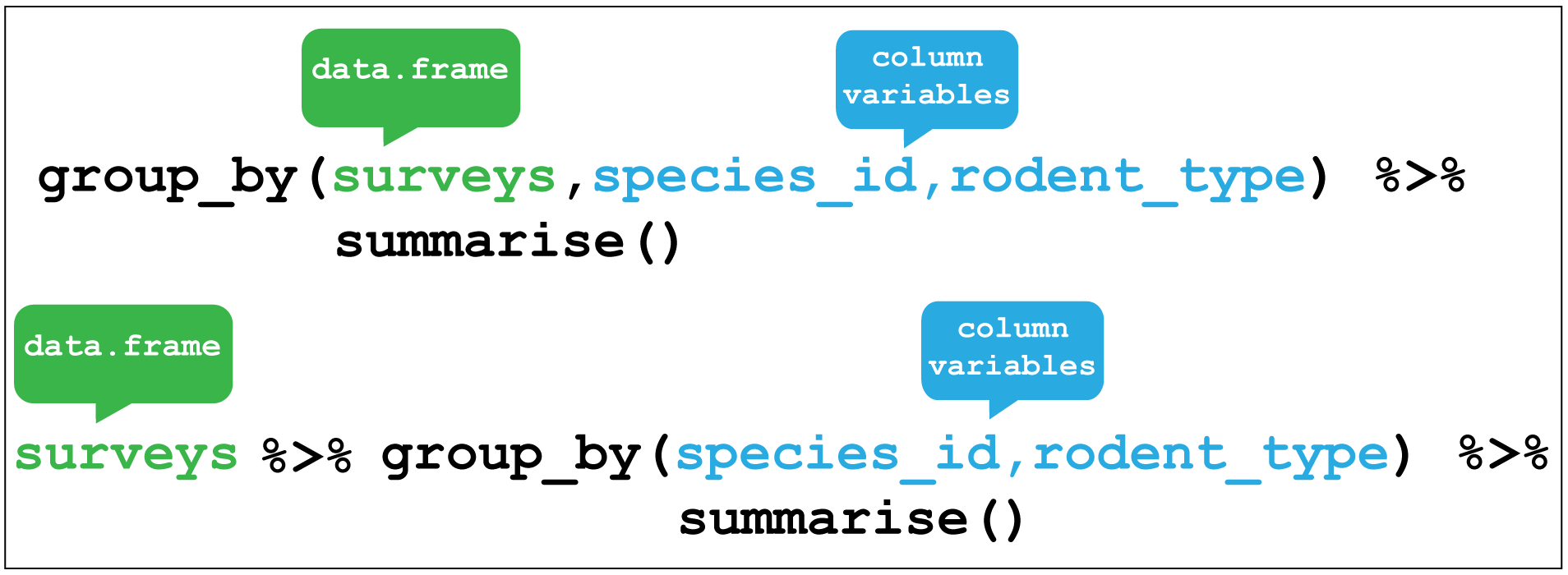
#> 1       42.67243

summarise() is most useful when paired with group_by() which defines the variables upon which we operate upon.

In the previous section we used this pairing to check when the species were correctly assigned their rodent type. We first grouped species_id and rodent_type together and then used summarise() without any arguments to show a summary of these two variables only.

# Check the output using a summary pipe, we should have 8 species of 2 types
surveys_mutate_rodent %>% group_by(species_id,rodent_type) %>% 
  summarise()

#> Source: local data frame [8 x 2]
#> Groups: species_id [?]
#> 
#>   species_id  rodent_type
#>        <chr>        <chr>
#> 1         DM Kangaroo Rat
#> 2         DO Kangaroo Rat
#> 3         DS Kangaroo Rat
#> 4         PE    Granivore
#> 5         PF    Granivore
#> 6         PM    Granivore
#> 7         PP    Granivore
#> 8         RM    Granivore

Let’s re-cap what we’ve done so far, and remind ourselves of the question we’re trying to answer:

Q: Is there evidence that kangaroo rats compete directly with four other granivore rodent species?

The evidence we are examining is the monthly populations of 8 species surveyed in four plots over a period of about 13 years. The initial dataset contains data about 40 species in 20 plots measuring 13 variables over 25 years.

At this point we have:

• Filtered the observations for the time period of interest, and for the species and plots of interest.
• We’ve created new variables for the rodent type, the date, and the year quarter
• We’ve selected only the variables we need to answer the question.

This reduces the dataset from around 35,000 observations of 13 variables to around 5,000 observations of 13 variables. We dropped three of the original variables and create three new variables.

We could start plotting the data, but it would be useful to summarise this a bit more. Concretely, we’d like to summarise the kangaroo rat and granivore populations on a monthly or quarterly basis. Or by genus.

This is where grouped summaries are very useful.

Grouping simply means grouping the variables of interest that we want to operate on, here they are the rodent_type (kangaroo rat and granivore), the quarter (the time period) and the plot_type (kangaroo rat exclusion or control). The summary we would like is the number of captures for each group e.g. number of captures of kangaroo rats for the first quarter of 1980 in the control plots. As each row in the table corresponds with a capture, we just need to count the number of rows in each group. We can do this using the count function n() in conjunction with summarise. This creates a new variable, a column containing the number of rows counted per group, which we’ll call captures. captures.

Here we have the additional issue that the grouping by quarter groups three months worth of captures, so to get the quarterly average number of captures we divide the number of rows counted by three.

# Summarise the data by rodent type, quarterly survey and plot type
by_quarter <- surveys_subset %>% 
  group_by(rodent_type,quarter,plot_type) %>% 
  summarise(captures = n()/3) 

glimpse(by_quarter)

#> Observations: 185
#> Variables: 4
#> $ rodent_type <chr> "Granivore", "Granivore", "Granivore", "Granivore"...
#> $ quarter     <dbl> 1977.3, 1977.3, 1977.4, 1977.4, 1978.1, 1978.2, 19...
#> $ plot_type   <chr> "Control", "Long-term Krat Exclosure", "Control", ...
#> $ captures    <dbl> 2.3333333, 0.6666667, 1.3333333, 1.0000000, 1.0000...

We have now transformed the dataset from a 35,000 observations of 13 variables table to the 185 observations of 4 variables table that we need for re-creating the plot shown in the paper.

Compare the output of glimpse(surveys) to glimpse(by_quarter).

But, this is not the only way to look at the data, so we’ll keep the unsummarised subset too. We could export the subset for sharing, but generally it’s better to share the raw data (if it’s not too large) and a script containing the code that will reproduce your transformations. Raw data is the form you received it in, it doesn’t necessarily mean that the data hasn’t been manipulated upstream.

We’ll finish this lesson with a challenge that uses the transformed data and rolls it up into 4 observations of 3 variables data frame by sucessive use of grouping and summarising.

Challenge

Use the group_by() and summarise() functions successively to examine whether the exclosure of kangaroo rats is successful or not.

First calculate the monthly captures per rodent type and plot type, then the yearly captures, and finally the total captures:

1. Create a summary data frame of surveys_subset called per_month grouping by rodent_type ,plot_type, year and month. Pipe the output to summarise() to create a new variable that calculates the monthly captures for each genus by replacing _ in summarise(montly = _) with the row counting function n().
2. Create a per_year data frame, using per_month with summarise() to create a yearly variable that sums the monthly captures. Provide per_month and sum(monthly) as the arguments to summarise().
3. Finally create a total data frame, summing the total caputures per rodent type and plot type by providing per_year and and sum(yearly) as the arguments to summarise().

Inspect total to see if the number of captures indicates whether the exlosure works to keep kangaroo rats out.

See SQL aggregation lesson to compare using dplyr in R with creating grouped summaries in SQL.