Learning Objectives

By the end of this lesson the learner will have:

Created an initial script for the analysis of the rodent survey data, and run the code they have written.

Downloaded and imported the survey data into a data frame using the download.file() function and the read_csv() function from the readr package.

Examined the structure of the imported data using the glimpse() function.

Seen what tidy data looks like, and inspected the data in detail to answer some basic queations about what the dataset contains.

In the remaining lessons we are going to recapitulate some of the analysis found in the 1994 paper by Heske et. al:

Long-Term Experimental Study of a Chihuahuan Desert Rodent Community: 13 Years of Competition, DOI: 10.2307/1939547.

Specifically we are going to look at the effect on the populations of small seed eating rodents as a result of the exclusion of larger competitor kangaroo rats over a period from 1977 to 1991.

Below is an image of one of the species of kangaroo rats excluded during the study.

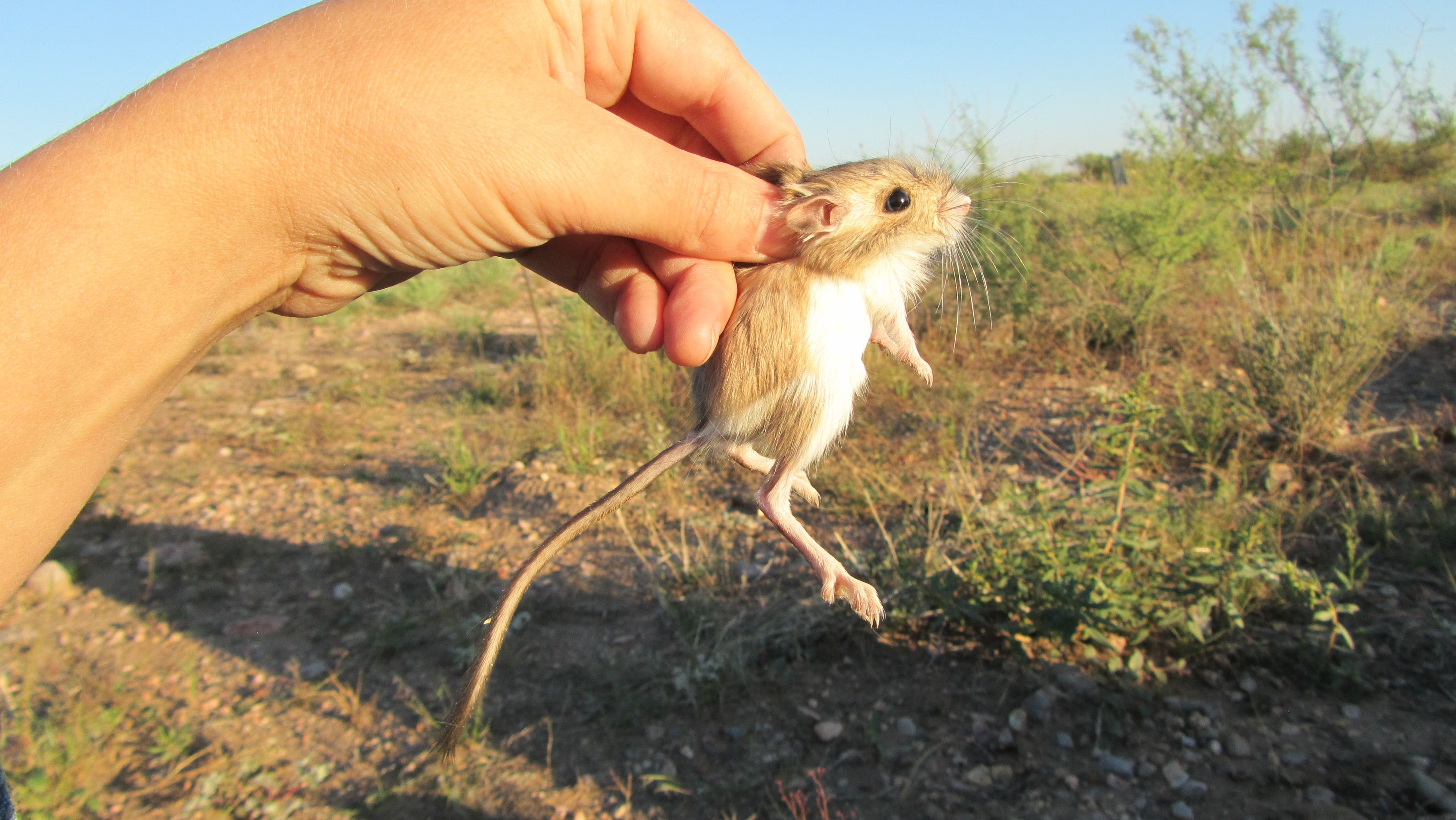
Merriam’s kangaroo rat, Dipodomys merriami, (https://portalproject.wordpress.com/)

Here is one of the smaller species whose populations were not excluded:

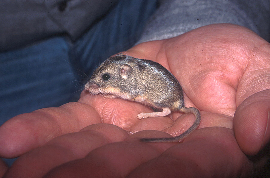
Silky pocket mouse,Perognathus flavus

The following image indicates how the exclusion works, where a for number of fenced plots the kangaroo rats were either able to enter by a hole or kept out.

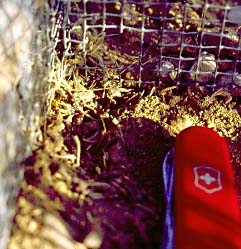
Kangeroo Rat exclusion

The plots are 50 metres by 50 metres, and a survey of the species within each plot has been ongoing once a month for many years.

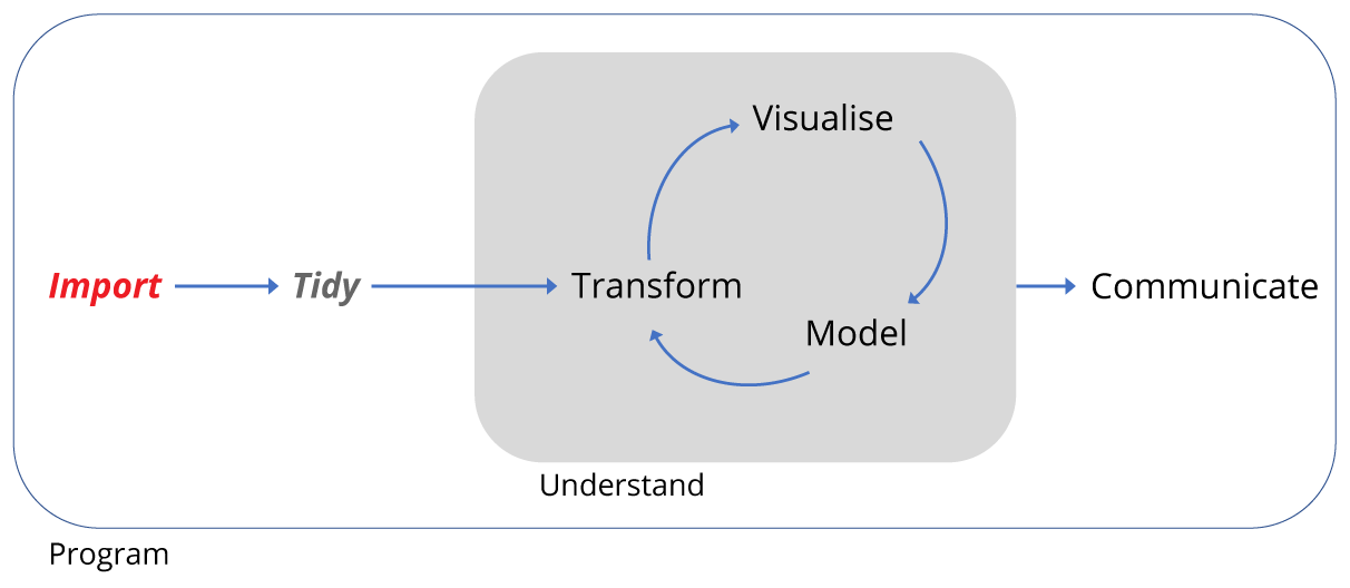
Here will practice importing data, transforming data, and plotting data, and finally turning this script into a report.

A conclusion of the paper is that there is evidence that kangaroo rats compete directly with four other rodent species, as evidenced by an increase in the populations of these four species when kangaroo Rats are excluded. This can be seen in Figure 1 in the paper, and we will try to reproduce the analysis to generate a similar figure and confirm these observations.

This figure shows the number of captures of threes species of kangaroo Rats and five species of smaller granivore rodents over a period from 1977 to 1990. Panel A shows the populations when the eight species were left to compete for resources and Panel B shows the effect of excluding the kangaroo Rats.

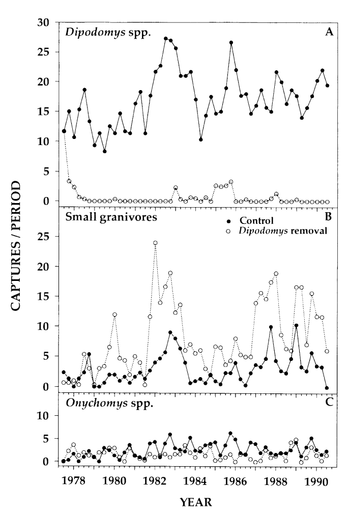
Figure 1 from Heske et. al., 1994

Importing and inspecting data

First we will learn how to download, import and inspect the rodent survey data, and the meaning of tidy data.

Importing means getting data into our R environment by turning into into a R object that we can then manipulate. The raw data file remains unchanged.
Inspecting means looking at the dataset to understand what it contains.
Tidying refers to getting data into a consistent format that makes it easy to use in later steps.

A note here is that we are focusing on rectangular data, the sort that comes in rows and columns such as in a spreadsheet. Lots of our data types exist, such as images, which are beyond the scope of this lesson, but can also be handled by R.

A further note on tidy data. Tidy data can also come in various forms, but for rectangular data we will use the convention where every variable forms a column, every row forms an observation and every type of observational unit is stored in a separate table (we only have one table here, so the last point is moot.) Data tidying can be done in R or elsewhere.

See the Data Organisation in Spreadsheets lesson for more about organising data so that it is tidy prior to importing to R.

Using scripts

Using the console is useful, but as we build up a workflow, that is to say, wring code to:

load packages
load data
explore the data
and output some results

Then it’s much more useful to contain this in a script: a document of our code.

Why? When we write and save our code in scripts, we can re-use it, share it or edit it. But most importantly a script is a record.

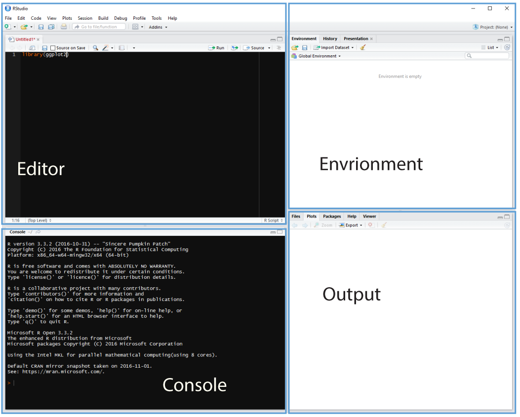
Cmd/Ctrl + Shift + N will open a new script file up and you should see something like below with the script editor pane open:

Running code

We can run a highlighted portion of code in your script if you click the Run button at the top of the scripts pane.

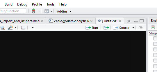
You can run the entire script by clicking the Source button.

Or we can run chunks of code if we split our script into sections, see below.

Creating a R script

We first need to create a script that will form the basis of our analysis.

Go to the file menu and select New Files > R script. This should open the script editor pane.

Now let’s save the script, by going to File > Save and we should find ourselves prompted to save the script in our Project Directory.

Filenames

File names should be meaningful and end in .R. A good name would be ecology-data-analysis.R and a bad name would be file.R. Let’s use the good example for our file name.

Comments

In R, any line beginning # is a comment line. Comments all your code to explain (to yourself) what is happening. The script can be turned into a report so the more comments you add the more time you save later on.

Starting on line 1, let’s put comment lines for the script title, our name and date.

# Ecology data analysis
# My name and today's date

Line length

It’s a good idea to keep lines to 80 characters to help make the code easy to read. You can display a margin from the Tools menu to show where 80 characters ends.

Code sections

We don’t always want to run the entire script, so it’s useful to split our script into sections, or code regions. Any comment line which includes at least four trailing dashes (-), equal signs (=), or hash/pound signs (#) to automatically creates a code section:

# This is a comment

# The dashes create a code region ----

# Let's create a character object called myName here:
myName <- "Alistair"

# Equals signs also create another code region =====

# And hash/pound symbols also create code regions ####

We can run each region separately, or the entire thing.

Setting up our R environment

We only need the tidyverse library, which contains all the packages we need for our analysis, so we add this to our script as before:

# Load the tidyverse set of packages -------------------------------------------
library(tidyverse)

Downloading and importing data

Downloading the rodent survey data from the web

Often you’ll be working with data you’ve generated and stored locally, but you may need to download data on occasion.

This gives us the chance to practice creating objects and try out using function with a condition.

First we’ll write a comment and create a code section at the same time. This is so we know what this code does, and so we can just run this bit of code easily.
Next we create the url object containing the web address of the data we need.
We also need a path object containing the address of where we want to download the data to and what to call the file. In this case it is the data folder we created and we will call it portal_data_joined.csv.
Then we use an if statement combined with a condition with the logical (TRUE/FALSE) file.exists() function to decide whether or not to download the data. The NOT condition ! means if portal_data_joined.csv doesn’t exist already, download it.

# Download the and import the data ---------------------------------------------

# First we assign the web address as a string to a R object called 'url'.
# Then we assign another string object called 'path' that states where we 
# want to import the data to.
# Next we use and 'if not' statement to check if the data has alredy been 
# downloaded. The '!' in front of 'file.exists' is a logical operator for 'not'.
# If there is no file called 'portal_data_joined.csv' in the 'data' folder,
# download the file.

# URL for portal joined survey data
url <- "https://ndownloader.figshare.com/files/2292169"
# Path and filename for downloading
path <- "data/portal_data_joined.csv"

# Check if the file exists, and if not download it to the data folder
if (!file.exists(path)) { download.file(url,path) }

Importing data using `readr`

Now we have downloaded it (check your data folder) we need to import it. As we have the tidyverse packages we can use the readr package it contains, which has many functions for reading files, including read_csv()

# Next we import the data using the 'readr' package and 'read_csv' function
# We'll assign the data to a R object called 'surveys'. 
# read_csv creates a 'tibble' a modified form of data frame with enhanced
# printing and checking capabilites.
surveys <- read_csv('data/portal_data_joined.csv')

## Parsed with column specification:
## cols(
##   record_id = col_integer(),
##   month = col_integer(),
##   day = col_integer(),
##   year = col_integer(),
##   plot_id = col_integer(),
##   species_id = col_character(),
##   sex = col_character(),
##   hindfoot_length = col_integer(),
##   weight = col_integer(),
##   genus = col_character(),
##   species = col_character(),
##   taxa = col_character(),
##   plot_type = col_character()
## )

The read_csv() function outputs a message telling us how it interpreted each column of data and what data type it stored them as. We can override these settings if needed, see the help file for more information ?read_csv.

A note on Excel files

The best way to move data from Excel to R is to export the spreadsheet from Excel as either a .csv or .txt file. These formats can be used with most data analysis software.

However, readxl is a tidyverse package that can be used for importing excel files to R.

Usage instructions can be found here: http://readxl.tidyverse.org/

Inspecting the dataset

Having imported the data, we should look at the structure of the data. We’ll use the glimpse function that tries to provide the most compact and informative view. The arguement we supply to glimpse is the surveys object we created in our environment when we imported the data.

# Inspect the data with 'glimpse'
glimpse(surveys)

## Observations: 34,786
## Variables: 13
## $ record_id       <int> 1, 72, 224, 266, 349, 363, 435, 506, 588, 661,...
## $ month           <int> 7, 8, 9, 10, 11, 11, 12, 1, 2, 3, 4, 5, 6, 8, ...
## $ day             <int> 16, 19, 13, 16, 12, 12, 10, 8, 18, 11, 8, 6, 9...
## $ year            <int> 1977, 1977, 1977, 1977, 1977, 1977, 1977, 1978...
## $ plot_id         <int> 2, 2, 2, 2, 2, 2, 2, 2, 2, 2, 2, 2, 2, 2, 2, 2...
## $ species_id      <chr> "NL", "NL", "NL", "NL", "NL", "NL", "NL", "NL"...
## $ sex             <chr> "M", "M", NA, NA, NA, NA, NA, NA, "M", NA, NA,...
## $ hindfoot_length <int> 32, 31, NA, NA, NA, NA, NA, NA, NA, NA, NA, 32...
## $ weight          <int> NA, NA, NA, NA, NA, NA, NA, NA, 218, NA, NA, 2...
## $ genus           <chr> "Neotoma", "Neotoma", "Neotoma", "Neotoma", "N...
## $ species         <chr> "albigula", "albigula", "albigula", "albigula"...
## $ taxa            <chr> "Rodent", "Rodent", "Rodent", "Rodent", "Roden...
## $ plot_type       <chr> "Control", "Control", "Control", "Control", "C...

This data is tidy already: each variable is a column, each observation is a row and each cell contains a single variable.

See the Data Organisation in Spreadsheets lessons for more about organising data so that it is tidy prior to importing to R.

There are a number of questions we might want to ask, such as:

Is there missing data?
How long a period does the dataset cover?
How many different taxa are there? (taxa are organism types e.g. plants or birds)
How many species are there? (individual species belong in their taxa)

For this analysis we need only the data required to create the plots that appear in the paper. This means subsetting surveys to keep only the species and taxa that were analysed, the time period of the experiment, and if necessary, remove any missing data.

Challenge

This challenge can be done in the console, or you can add your code to your script if you prefer.

Is there missing data? (R uses NA to represent missing values.)

How long a period does the dataset cover?

HINT: columns in a data.frame can be accessed using $ sign in the form data_frame$column_name HINT: try the range() function on the year column.

How many different taxa are there? (taxa are organism types e.g. plants or birds)

HINT: try the distinct() function to find the unique values for taxa. This function is takes arguments of the form distinct(data_frame,column_name).

How many species are there? (Use distinct again, but this time add %>% count() to the end of the command. This pipes the output of distinct to the count() function)

Data Carpentry, 2017.
License. Questions? Feedback? Please file an issue on GitHub.
On Twitter: @datacarpentry

Importing and inspecting data

Alistair Bailey

Learning Objectives

Importing and inspecting data

Using scripts

Running code

Creating a R script

Filenames

Comments

Line length

Code sections

Setting up our R environment

Downloading and importing data

Downloading the rodent survey data from the web

Importing data using readr

A note on Excel files

Inspecting the dataset

Challenge

Importing data using `readr`