Working Environment

Learning Objectives

Working Environment

Describe the purpose of the RStudio Script, Console, Environment, and Plots panes.

Organize files and directories for a set of analyses as an R Project, and understand the purpose of the working directory.

Use the built-in RStudio help interface to search for more information on R functions.

R Basics

Define the following terms as they relate to R: object, assign, call, function, arguments, options.

Create objects and assign values to them in R.

Learn how to name objects

Use comments to inform script.

Solve simple arithmetic operations in R.

Call functions and use arguments to change their default options.

Inspect the content of vectors and manipulate their content.

Subset and extract values from vectors.

Analyze vectors with missing data.

Load Data

Load external data from a .csv file into a data frame.

Describe what a data frame is.

Summarize the contents of a data frame.

Use indexing to subset specific portions of data frames.

Format dates.

To start with we will focus on the first three learning objectives and get your working environment set up.

What is R? What is RStudio?

The term “R” is used to refer to both the programming language and the software that interprets the scripts written using it.

RStudio is a very popular way to not only write R scripts but also to interact with the R software. To function correctly, RStudio needs R and therefore both need to be installed on your computer.

Why learn R?

R does not involve lots of pointing and clicking, and that’s a good thing

The learning curve might be steeper than with other software, but with R, the results of your analysis do not rely on a succession of pointing and clicking, but instead on a series of written commands, and that’s a good thing! So, if you want to redo your analysis because you collected more data, you don’t have to remember which button you clicked in which order to obtain your results; you just have to run your script again.

Working with scripts makes the steps you used in your analysis clear, and the code you write can be inspected by someone else who can give you feedback and spot mistakes.

Working with scripts enables a deeper understanding of what you are doing, and facilitates your learning and comprehension of the methods you use.

R code is great for reproducibility

Reproducibility is when someone else (including your future self) can obtain the same results from the same dataset when using the same analysis.

An increasing number of journals and funding agencies expect analyses to be reproducible, so knowing R will give you an edge with these requirements.

R is interdisciplinary and extensible

With 10,000+ packages that can be installed to extend its capabilities, R provides a framework to best suit the analytical framework you need to analyze your data. For instance, R has packages for image analysis, GIS, time series, population genetics, and a lot more.

R works on data of all shapes and sizes

The skills you learn with R scale easily with the size of your dataset. Whether your dataset has hundreds or millions of lines, it won’t make much difference to you.

R is designed for data analysis. It comes with special data structures and data types that make handling of missing data and statistical factors convenient.

R can connect to spreadsheets, databases, and many other data formats, on your computer or on the web.

R produces high-quality graphics

The plotting functionalities in R are endless, and allow you to adjust any aspect of your graph to convey most effectively the message from your data.

R has a large and welcoming community

Thousands of people use R daily. Many of them are willing to help you through mailing lists and websites such as Stack Overflow, or on the RStudio community.

Knowing your way around RStudio

Let’s start by learning about RStudio, which is an open-source Integrated Development Environment (IDE) for working with R.

We will use RStudio IDE to write code, navigate the files on our computer, inspect the variables we are going to create, and visualize the plots we will generate.

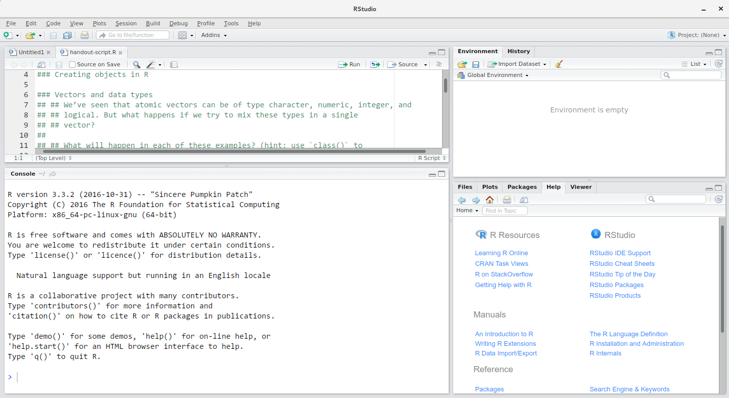
RStudio interface screenshot. Clockwise from top left: Source, Environment/History, Files/Plots/Packages/Help/Viewer, Console.

RStudio is divided into 4 “Panes”: the Source for your scripts and documents (top-left, in the default layout), your Environment/History (top-right) which shows all the objects in your working space (Environment) and your command history (History), your Files/Plots/Packages/Help/Viewer (bottom-right), and the R Console (bottom-left). The placement of these panes and their content can be customized (see menu, Tools -> Global Options -> Pane Layout).

Getting set up

It is good practice to keep a set of related data, analyses, and text self-contained in a single folder, called the working directory. All of the scripts within this folder can then use relative paths to files that indicate where inside the project a file is located. Working this way makes it a lot easier to move your project around on your computer and share it with others.

RStudio provides a helpful set of tools to do this through its “Projects” interface, which not only creates a working directory for you, but also remembers its location (allowing you to quickly navigate to it). Go through the steps for creating an “R Project” for this tutorial below.

Start RStudio.
Under the File menu, click on New Project. Choose New Directory, then New Project.
Enter a name for this new folder (or “directory”), and choose a convenient location for it. This will be your working directory for the rest of the day (e.g., ~/data-carpentry).
Click on Create Project.
(Optional) Set Preferences to ‘Never’ save workspace in RStudio.

A workspace is your current working environment in R which includes any user-defined object. By default, all of these objects will be saved, and automatically loaded, when you reopen your project. Saving a workspace to .RData can be cumbersome, especially if you are working with larger datasets, and it can lead to hard to debug errors by having objects in memory you forgot you had. To turn that off, go to Tools –> ‘Global Options’ and select the ‘Never’ option for ‘Save workspace to .RData’ on exit.’

Set ‘Save workspace to .RData on exit’ to ‘Never’

Stretch Challenge (Difficult - 1hr+)

Under the File menu, click on New Project and choose New Directory like before. Then investigate the other project structures that are available such as ‘Shiny Web Application’ or ‘R Package’. If you’re interested in either of these, have a look at this further information about making your own Shiny Web Application or R Package.

Organizing your working directory

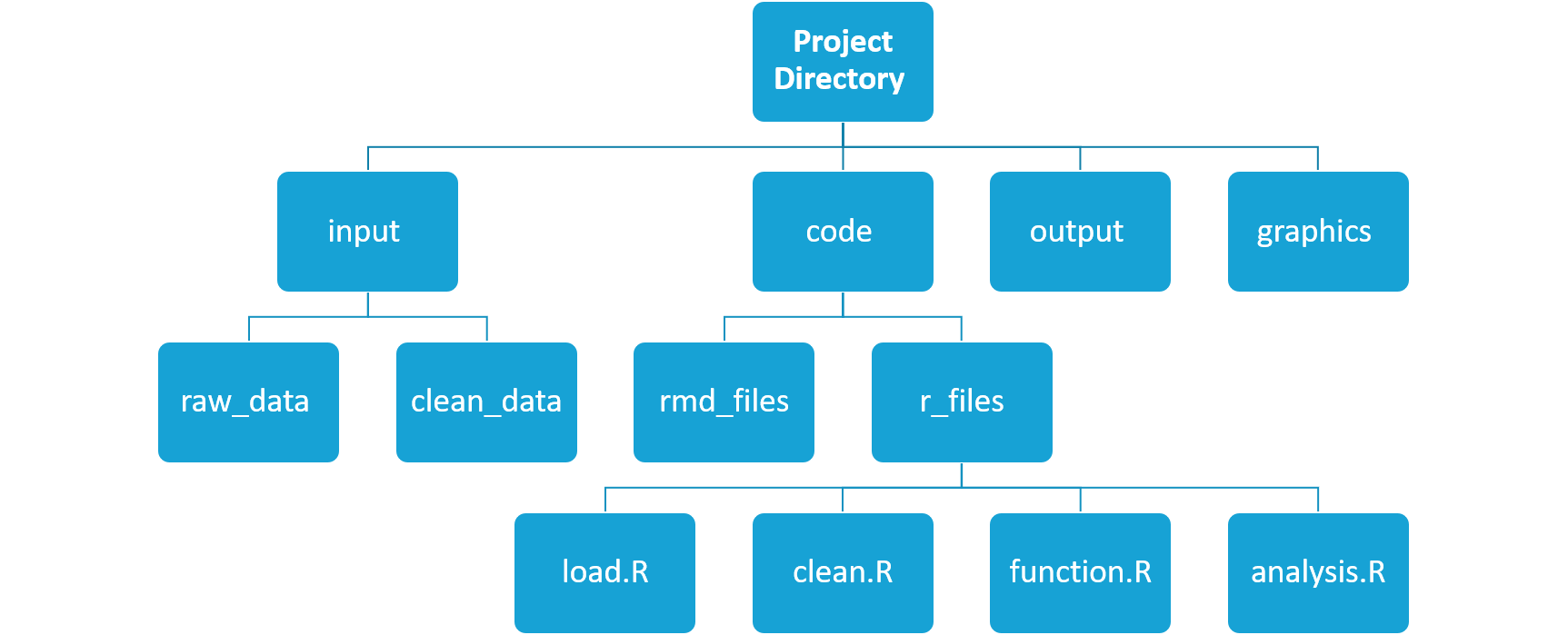
Using a consistent folder structure across your projects will make it easy to find/file things in the future. This can be especially helpful when you have multiple projects. In general, you may create directories (folders) for scripts, data, and documents.

data_raw/ & data/ Use these folders to store raw data and intermediate datasets you may create for the need of a particular analysis. For the sake of transparency and provenance, you should always keep a copy of your raw data accessible and do as much of your data cleanup and preprocessing programmatically (i.e., with scripts, rather than manually) as possible. Separating raw data from processed data is also a good idea. For example, you could have files data_raw/tree_survey.plot1.txt and ...plot2.txt kept separate from a data/tree.survey.csv file generated by the scripts/01.preprocess.tree_survey.R script.
documents/ This would be a place to keep outlines, drafts, and other text.
scripts/ This would be the location to keep your R scripts for different analyses or plotting, and potentially a separate folder for your functions (more on that later).
Additional (sub)directories depending on your project needs.

For this workshop, we will need a data_raw/ folder to store our raw data, and we will use data/ for when we learn how to export data as CSV files, and a fig/ folder for the figures that we will save.

Under the Files tab on the right of the screen, click on New Folder and create a folder named data_raw within your newly created working directory (e.g., ~/data-carpentry/). (Alternatively, type dir.create("data_raw") at your R console.) Repeat these operations to create a data and a fig folder.

We are going to keep the script in the root of our working directory because we are only going to use one file and it will make things easier. Create this using the new file button in the top left hand corner and select R Script, the hit save and name it data-carpentry-script.

Your working directory should now look like this:

Stretch Challenge (Intermediate - 15 mins)

Try creating the file structure shown below using only commands in the R console.

The working directory

The working directory is an important concept to understand. It is the place from where R will be looking for and saving the files. When using R projects the working directory has a .Rproj file in it. When you write code for your project, it should refer to files in relation to the root of your working directory and only need files within this structure.

Using RStudio projects makes this easy and ensures that your working directory is set properly. If you need to check it, you can use getwd(). If for some reason your working directory is not what it should be, you can change it in the RStudio interface by navigating in the file browser where your working directory should be, and clicking on the blue gear icon “More”, and select “Set As Working Directory”. Alternatively you can use setwd("/path/to/working/directory") to reset your working directory. However, your scripts should not include this line because it will fail on someone else’s computer.

Interacting with R

The basis of programming is that we write down instructions for the computer to follow, and then we tell the computer to follow those instructions. We write, or code, instructions in R because it is a common language that both the computer and we can understand. We call the instructions commands and we tell the computer to follow the instructions by executing (also called running) those commands.

There are two main ways of interacting with R: by using the console or by using script files (plain text files that contain your code). The console pane (in RStudio, the bottom left panel) is the place where commands written in the R language can be typed and executed immediately by the computer. It is also where the results will be shown for commands that have been executed. You can type commands directly into the console and press Enter to execute those commands, but they will be forgotten when you close the session.

Because we want our code and workflow to be reproducible, it is better to type the commands we want in the script editor, and save the script. This way, there is a complete record of what we did, and anyone (including our future selves!) can replicate the results on their computer.

RStudio allows you to execute commands directly from the script editor by using the Ctrl + Enter shortcut (on Macs, Cmd + Return will work, too). The command on the current line in the script (indicated by the cursor) or all of the commands in the currently selected text will be sent to the console and executed when you press Ctrl + Enter. You can find other keyboard shortcuts in this RStudio cheatsheet about the RStudio IDE.

If R is ready to accept commands, the R console shows a > prompt. If it receives a command (by typing, copy-pasting or sent from the script editor using Ctrl + Enter), R will try to execute it, and when ready, will show the results and come back with a new > prompt to wait for new commands.

If R is still waiting for you to enter more data because it isn’t complete yet, the console will show a + prompt. It means that you haven’t finished entering a complete command. This is because you have not ‘closed’ a parenthesis or quotation, i.e. you don’t have the same number of left-parentheses as right-parentheses, or the same number of opening and closing quotation marks. When this happens, and you thought you finished typing your command, click inside the console window and press Esc; this will cancel the incomplete command and return you to the > prompt.

Seeking help

Use the built-in RStudio help interface to search for more information on R functions

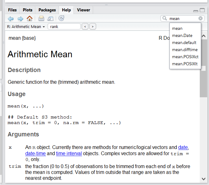
RStudio help interface.

One of the fastest ways to get help, is to use the RStudio help interface. This panel by default can be found at the lower right hand panel of RStudio. As seen in the screenshot, by typing the word “Mean”, RStudio tries to also give a number of suggestions that you might be interested in. The description is then shown in the display window.

I know the name of the function I want to use, but I’m not sure how to use it

If you need help with a specific function, let’s say lm(), you can type:

?lm

I want to use a function that does X, there must be a function for it but I don’t know which one…

If you are looking for a function to do a particular task, you can use the help.search() function, which is called by the double question mark ??. However, this only looks through the installed packages for help pages with a match to your search request

??kruskal

If you can’t find what you are looking for, you can use the rdocumentation.org website that searches through the help files across all packages available.

Finally, a generic Google or internet search “R <task>” will often either send you to the appropriate package documentation or a helpful forum where someone else has already asked your question.

I am stuck… I get an error message that I don’t understand

Start by googling the error message. However, this doesn’t always work very well because often, package developers rely on the error catching provided by R. You end up with general error messages that might not be very helpful to diagnose a problem (e.g. “subscript out of bounds”). If the message is very generic, you might also include the name of the function or package you’re using in your query.

Where to ask for help?

The other people here; you might also be interested in organizing regular meetings following the workshop to keep learning from each other.
Your friendly colleagues: if you know someone with more experience than you, they might be able and willing to help you.
Stack Overflow’s [r]-tag: Most questions have already been answered, but the challenge is to use the right words in the search to find the answers. If your question hasn’t been answered before and is well crafted, chances are you will get an answer in less than 5 min. Remember to follow their guidelines on how to ask a good question.

Page built on: <U+0001F4C6> 2021-09-14 - <U+0001F562> 16:08:43

R Basics

Learning Objectives: Recap

Working Environment: Done

~~Describe the purpose of the RStudio Script, Console, Environment, and Plots~~ ~~panes.~~

~~Organize files and directories for a set of analyses as an R~~ ~~Project, and understand the purpose of the working directory.~~

~~Use the built-in RStudio help interface to search for more information on R~~ ~~functions.~~

R Basics

Define the following terms as they relate to R: object, assign, call, function, arguments, options.

Create objects and assign values to them in R.

Learn how to name objects

Use comments to inform script.

Solve simple arithmetic operations in R.

Call functions and use arguments to change their default options.

Inspect the content of vectors and manipulate their content.

Subset and extract values from vectors.

Analyze vectors with missing data.

Load Data

Load external data from a .csv file into a data frame.

Describe what a data frame is.

Summarize the contents of a data frame.

Use indexing to subset specific portions of data frames.

Format dates.

Now that we have a working environment set up we can start on the basics of R.

Creating objects in R

You can get output from R simply by typing math in the console:

3 + 5
12 / 7

Stretch Challenge (Intermediate - 15 mins)

Using the information above about how and where to ask a question online, find out the r arithmetic operators for the following operations:
Remainder from integer division (modulus) e.g. remainder of 8/3
Answer
8 %% 3
Raise to the power of (exponentiation) e.g. 5 to the power of 2
Answer
5 ^ 2

However, to do useful and interesting things, we need to assign values to objects.

A value is a piece of information that we want to store and retrieve at some later time, i.e. a number, a sequence of numbers, or even collections of data, for now we will start with numbers and later move onto collections of numbers which in R are called vectors.

An object is programming speak for a thing with known properties. Lets consider an example that we would all be familiar with before jumping into some R.

I tell you that I have a car, in this case the car is the object. Without any further information you instinctivly know that the object called car has several attributes. For example, colour, make, model, numberplate. You can use this predefined model to ask sensible questions. For example if you ask me, what model the car is (or model(car)) I can tell you ‘Corsa’. However, if you were to ask me breed(car) this would be a nonsense question to which I would not be able to answer, where as breed(pet) then I could tell you ‘sheepdog’.

Challenge
Write down three other attributes for the object pet?

Answer

Including but not limited to: Species, Age, Colour, Name, Sex, Owner…

In this tutorial we will use the predefined R objects for vectors and numerical values. We will see that these are much simpler than the linguistic examples above, and we learn the sort of attributes we expect them to have and how to inspect an object to tell us its set of attributes.

To create an object, we need to give it a name followed by the assignment operator <-, and the value we want to give it:

weight_kg <- 55

<- is the assignment operator. It assigns values on the right to objects on the left. So, after executing weight_kg <- 55, the value of weight_kg is 55. The arrow can be read as 55 goes into weight_kg.

What is my object?

Once an object is created we can get information about that object in the Environment tab in the top right of RStudio. For example, ‘weight_kg’ has the type numeric length 1 and value 55. Make sure to keep an eye on the other values that appear here when using RStudio to understand what objects you have. This tab is great for small variables, when inspecting larger or more complicated objects it is better to use more advanced methods we will cover later on.

How do I name my objects?

Objects can be given any name such as x, current_temperature, or subject_id. You want your object names to be explicit and not too long. They cannot start with a number (2x is not valid, but x2 is). R is case sensitive (e.g., weight_kg is different from Weight_kg). There are some names that cannot be used because they are the names of fundamental functions in R (e.g., if, else, for, see here for a complete list). In general, even if it’s allowed, it’s best to not use other function names (e.g., c, T, mean, data, df, weights). If in doubt, check the help to see if the name is already in use. It’s also best to avoid dots (.) within names. Many function names in R itself have them and dots also have a special meaning (methods) in R and other programming languages. To avoid confusion, don’t include dots in names. It is also recommended to use nouns for object names, and verbs for function names. It’s important to be consistent in the styling of your code (where you put spaces, how you name objects, etc.). Using a consistent coding style makes your code clearer to read for your future self and your collaborators. In R, three popular style guides are Google’s, Jean Fan’s and the tidyverse’s. The tidyverse’s is very comprehensive and may seem overwhelming at first. You can install the lintr package to automatically check for issues in the styling of your code.

Objects vs. variables

What are known as objects in R are known as variables in many other programming languages. Depending on the context, object and variable can have drastically different meanings. However, in this lesson, the two words are used synonymously. For more information see: https://cran.r-project.org/doc/manuals/r-release/R-lang.html#Objects

When assigning a value to an object, R does not print anything. You can force R to print the value by using parentheses or by typing the object name:

weight_kg <- 55    # doesn't print anything
(weight_kg <- 55)  # but putting parenthesis around the call prints the value of `weight_kg`
weight_kg          # and so does typing the name of the object

Now that R has weight_kg in memory, we can do arithmetic with it. For instance, we may want to convert this weight into pounds (weight in pounds is 2.2 times the weight in kg):

2.2 * weight_kg

#> [1] 121

We can also change an object’s value by assigning it a new one:

weight_kg <- 57.5
2.2 * weight_kg

#> [1] 126.5

This means that assigning a value to one object does not change the values of other objects. For example, let’s store the animal’s weight in pounds in a new object, weight_lb:

weight_lb <- 2.2 * weight_kg

and then change weight_kg to 100.

weight_kg <- 100

What do you think is the current content of the object weight_lb? 126.5 or 220?

Comments

The comment character in R is #, anything to the right of a # in a script will be ignored by R. It is best practice to leave notes and explanations in your scripts. So that others can understand your code and that you can remember what each line does.

Challenge

What are the values after each statement in the following?

mass <- 47.5            # mass?
age  <- 122             # age?
mass <- mass * 2.0      # mass?
age  <- age - 20        # age?
mass_index <- mass/age  # mass_index?

Functions and their arguments

Functions automate sets of commands including operations assignments, etc. Many functions are predefined, or can be made available by importing R packages (more on that later). A function usually takes one or more inputs called arguments. Functions often (but not always) return a value. A typical example would be the function sqrt(). The input (the argument) must be a number, and the return value (in fact, the output) is the square root of that number. Executing a function (‘running it’) is called calling the function. An example of a function call is:

weight_kg <- sqrt(10)

Here, the value of ten is given to the sqrt() function, the sqrt() function calculates the square root, and returns the value which is then assigned to the object weight_kg. This function is very simple, because it takes just one argument.

The return ‘value’ of a function need not be numerical (like that of sqrt()), and it also does not need to be a single item: it can be a set of things, or even a dataset. We’ll see that when we read data files into R.

Arguments can be anything, not only numbers or filenames, but also other objects. Exactly what each argument means differs per function, and must be looked up in the documentation (see below). Some functions take arguments which may either be specified by the user, or, if left out, take on a default value: these are called options. Options are typically used to alter the way the function operates, such as whether it ignores ‘bad values’, or what symbol to use in a plot. However, if you want something specific, you can specify a value of your choice which will be used instead of the default.

Let’s try a function that can take multiple arguments: round().

round(3.14159)

#> [1] 3

Here, we’ve called round() with just one argument, 3.14159, and it has returned the value 3. That’s because the default is to round to the nearest whole number. If we want more digits we can see how to do that by getting information about the round function. We can use args(round) to find what arguments it takes, or look at the help for this function using ?round.

args(round)

#> function (x, digits = 0) 
#> NULL

?round

We see that if we want a different number of digits, we can type digits = 2 or however many we want.

round(3.14159, digits = 2)

#> [1] 3.14

Stretch Challenge (Intermediate - 10 mins)

Use args() to query the arguments for the functions used so far including dir.create(), mean(), and sqrt()

Use ? (e.g. ?length) to learn more about the functions and their arguments.

Write your own function and then inspect it using args(). You can use the basic function below as a template.
add_together <- function (x, y) {
   x + y
}

Vectors and data types

A vector is the most common and basic data type in R. A vector is composed by a series of values, which can be either numbers or characters. We can assign a series of values to a vector using the c() function. For example we can create a vector of animal weights and assign it to a new object weight_g:

weight_g <- c(50, 60, 65, 82)
weight_g

#> [1] 50 60 65 82

A vector can also contain characters:

animals <- c("mouse", "rat", "dog")
animals

#> [1] "mouse" "rat"   "dog"

The quotes around “mouse”, “rat”, etc. are essential here to tell R that these are characters and not objects.

There are many functions that allow you to inspect the content of a vector. length() tells you how many elements are in a particular vector:

length(weight_g)

#> [1] 4

length(animals)

#> [1] 3

An important feature of a vector, is that all of the elements are the same type of data. The function class() indicates what kind of object you are working with:

class(weight_g)

#> [1] "numeric"

class(animals)

#> [1] "character"

The function str() provides an overview of the structure of an object and its elements. It is a useful function when working with large and complex objects:

str(weight_g)

#>  num [1:4] 50 60 65 82

str(animals)

#>  chr [1:3] "mouse" "rat" "dog"

You can use the c() function to add other elements to your vector:

weight_g <- c(weight_g, 90) # add to the end of the vector
weight_g <- c(30, weight_g) # add to the beginning of the vector
weight_g

#> [1] 30 50 60 65 82 90

In the first line, we take the original vector weight_g, add the value 90 to the end of it, and save the result back into weight_g. Then we add the value 30 to the beginning, again saving the result back into weight_g.

We can do this over and over again to grow a vector, or assemble a dataset. As we program, this may be useful to add results that we are collecting or calculating.

An atomic vector is the simplest R data type and is a linear vector of a single type. The 6 atomic vector types are:

"character" for text
"numeric" or "double" for non-interger numbers
"logical" for TRUE and FALSE (the boolean data type)
"integer" for integer numbers (e.g., 2L, the L indicates to R that it’s an integer)
"complex" to represent complex numbers with real and imaginary parts (e.g., 1 + 4i) and that’s all we’re going to say about them
"raw" for bitstreams that we won’t discuss further

You can check the type of your vector using the typeof() function and inputting your vector as the argument.

Vectors are one of the many data structures that R uses. Other important ones are lists (list), matrices (matrix), data frames (data.frame), factors (factor) and arrays (array).

Challenge

We’ve seen that atomic vectors can be of type character, numeric (or double), integer, and logical. But what happens if we try to mix these types in a single vector?

Answer

R implicitly converts them to all be the same type
What will happen in each of these examples? (hint: use class() to check the data type of your objects):
num_char <- c(1, 2, 3, "a")
num_logical <- c(1, 2, 3, TRUE)
char_logical <- c("a", "b", "c", TRUE)
tricky <- c(1, 2, 3, "4")
Why do you think it happens?
Answer

Vectors can be of only one data type. R tries to convert (coerce) the content of this vector to find a “common denominator” that doesn’t lose any information.
How many values in combined_logical are "TRUE" (as a character) in the following example (reusing the 2 ..._logicals from above):
combined_logical <- c(num_logical, char_logical)
Answer

Only one. There is no memory of past data types, and the coercion happens the first time the vector is evaluated. Therefore, the TRUE in num_logical gets converted into a 1 before it gets converted into "1" in combined_logical.

You’ve probably noticed that objects of different types get converted into a single, shared type within a vector. In R, we call converting objects from one class into another class coercion. These conversions happen according to a hierarchy, whereby some types get preferentially coerced into other types. Can you draw a diagram that represents the hierarchy of how these data types are coerced?

Answer

logical → numeric → character ← logical

Stretch Challenge (Intermediate - 20 mins)

Look up the functions seq() and rep() Use these functions to create the following vectors:
1 2 3 4 5 1 2 3 4 5 1 2 3 4 5
Answer
 rep(1:5, 3)
3 6 9 12 15 18 21 24 27 30
Answer
seq(3, 30, 3)
Note: there are several possible solutions

Subsetting vectors

If we want to extract one or several values from a vector, we must provide one or several indices in square brackets. For instance:

animals <- c("mouse", "rat", "dog", "cat")
animals[2]

#> [1] "rat"

animals[c(3, 2)]

#> [1] "dog" "rat"

We can also repeat the indices to create an object with more elements than the original one:

more_animals <- animals[c(1, 2, 3, 2, 1, 4)]
more_animals

#> [1] "mouse" "rat"   "dog"   "rat"   "mouse" "cat"

Conditional subsetting

Another common way of subsetting is by using a logical vector. TRUE will select the element with the same index, while FALSE will not:

weight_g <- c(21, 34, 39, 54, 55)
weight_g[c(TRUE, FALSE, FALSE, TRUE, TRUE)]

#> [1] 21 54 55

Typically, these logical vectors are not typed by hand, but are the output of other functions or logical tests. For instance, if you wanted to select only the values above 50:

weight_g > 50    # will return logicals with TRUE for the indices that meet the condition

#> [1] FALSE FALSE FALSE  TRUE  TRUE

## so we can use this to select only the values above 50
weight_g[weight_g > 50]

#> [1] 54 55

You can combine multiple tests using & (both conditions are true, AND) or | (at least one of the conditions is true, OR):

weight_g[weight_g > 30 & weight_g < 50]

#> [1] 34 39

weight_g[weight_g <= 30 | weight_g == 55]

#> [1] 21 55

weight_g[weight_g >= 30 & weight_g == 21]

#> numeric(0)

Here, > for “greater than”, < stands for “less than”, <= for “less than or equal to”, and == for “equal to”. The double equal sign == is a test for numerical equality between the left and right hand sides, and should not be confused with the single = sign, which performs variable assignment (similar to <-).

A common task is to search for certain strings in a vector. One could use the “or” operator | to test for equality to multiple values, but this can quickly become tedious. The function %in% allows you to test if any of the elements of a search vector are found:

animals <- c("mouse", "rat", "dog", "cat")
animals[animals == "cat" | animals == "rat"] # returns both rat and cat

#> [1] "rat" "cat"

animals %in% c("rat", "cat", "dog", "duck", "goat")

#> [1] FALSE  TRUE  TRUE  TRUE

animals[animals %in% c("rat", "cat", "dog", "duck", "goat")]

#> [1] "rat" "dog" "cat"

Stretch Challenge (Difficult - 10 mins)

creatures <- c('rat', 'sheep','squirrel', 'tiger', 'whale', 'dolphin', 
               'jellyfish','octopus', 'shark') 
mammals <- c('rat', 'sheep','squirrel', 'tiger', 'whale', 'dolphin')
sea_creatures <- c('jellyfish', 'whale', 'octopus', 'shark', 'dolphin')

Create a vector of creatures that are either mammals or sea creatures but not both

Answer

 creatures[!(creatures %in% mammals & creatures %in% sea_creatures)]

Missing data

As R was designed to analyze datasets it includes the concept of missing data. Missing data are represented in vectors as NA.

When doing operations on numbers, most functions will return NA if the data you are working with include missing values. This feature makes it harder to overlook the cases where you are dealing with missing data. You can add the argument na.rm = TRUE to calculate the result while ignoring the missing values.

heights <- c(2, 4, 4, NA, 6)
mean(heights)
max(heights)
mean(heights, na.rm = TRUE)
max(heights, na.rm = TRUE)

If your data include missing values, you may want to become familiar with the functions is.na(), na.omit(), and complete.cases(). See below for examples.

## Extract those elements which are not missing values.
heights[!is.na(heights)]

## Returns the object with incomplete cases removed. 
#The returned object is an atomic vector of type `"numeric"` (or #`"double"`).
na.omit(heights)

## Extract those elements which are complete cases. 
#The returned object is an atomic vector of type `"numeric"` (or #`"double"`).
heights[complete.cases(heights)]

Recall that you can use the typeof() function to find the type of your atomic vector.

Challenge

Using this vector of heights in inches, create a new vector, heights_no_na, with the NAs removed.

heights <- c(63, 69, 60, 65, NA, 68, 61, 70, 61, 59, 64, 69, 63, 63, NA, 72, 65, 64, 70, 63, 65)

Use the function median() to calculate the median of the heights vector.
Use R to figure out how many people in the set are taller than 67 inches.

Answer

heights <- c(63, 69, 60, 65, NA, 68, 61, 70, 61, 59, 64, 69, 63, 63, NA, 72, 65, 64, 70, 63, 65)

# 1.
heights_no_na <- heights[!is.na(heights)] 
# or
heights_no_na <- na.omit(heights)
# or
heights_no_na <- heights[complete.cases(heights)]

# 2.
median(heights, na.rm = TRUE)

# 3.
heights_above_67 <- heights_no_na[heights_no_na > 67]
length(heights_above_67)

Now that we have learned how to write scripts, and the basics of R’s data structures, we are ready to start working with the Portal dataset we have been using in the other lessons, and learn about data frames.

Stretch Challenge (Fiendish - 1hr+)

Have a look at a package called mice for some more advanced methods of dealing with multivariate missing data.

Load Data

Learning Objectives: Recap

Working Environment: Done

~~Describe the purpose of the RStudio Script, Console, Environment, and Plots~~ ~~panes.~~

~~Organize files and directories for a set of analyses as an R~~ ~~Project, and understand the purpose of the working directory.~~

~~Use the built-in RStudio help interface to search for more information on R~~ ~~functions.~~

R Basics

~~Define the following terms as they relate to R: object, assign, call,~~ ~~function, arguments, options.~~

~~Create objects and assign values to them in R.~~

~~Learn how to name objects~~

~~Use comments to inform script.~~

~~Solve simple arithmetic operations in R.~~

~~Call functions and use arguments to change their default options.~~

~~Inspect the content of vectors and manipulate their content.~~

~~Subset and extract values from vectors.~~

~~Analyze vectors with missing data.~~

Load Data

Load external data from a .csv file into a data frame.

Describe what a data frame is.

Summarize the contents of a data frame.

Use indexing to subset specific portions of data frames.

Format dates.

We have now learnt enough of the basics of R to be able to use R in place of spreadsheets. As the previous lessons will have shown you spreadsheets can be good for small amounts of data that can be managed by hand. With R will will be able to load large sets of data and create readable, reliable, and reproducible data analysis scripts.

Presentation of the Survey Data

We are investigating the animal species diversity and weights found within plots at our study site. The dataset is stored as a comma separated value (CSV) file. Each row holds information for a single animal, and the columns represent:

Column	Description
record_id	Unique id for the observation
month	month of observation
day	day of observation
year	year of observation
plot_id	ID of a particular plot
species_id	2-letter code
sex	sex of animal (“M”, “F”)
hindfoot_length	length of the hindfoot in mm
weight	weight of the animal in grams
genus	genus of animal
species	species of animal
taxon	e.g. Rodent, Reptile, Bird, Rabbit
plot_type	type of plot

We are going to use the R function download.file() to download the CSV file that contains the survey data from Figshare. Lets investigate the download.file() function.

In the R console type ?download.file and then look at the help view that will open on the bottom right. We can see a description and a list of arguments. We need the first two, url and destfile.

url: A character string giving a source URL for the data we use “https://ndownloader.figshare.com/files/2292169”.

destfile: A character string (or vector) denoting the destination and name for the downloaded data we use “data_raw/portal_data_joined.csv”.

You’ll need the folder on your machine called “data_raw” in your working envronment which we made earlier. So this command downloads a file from Figshare, names it “portal_data_joined.csv” and adds it to the preexisting folder named “data_raw”.

download.file(url = "https://ndownloader.figshare.com/files/2292169",
              destfile = "data_raw/portal_data_joined.csv")

You are now ready to load the data we use read.csv() to load the content of the CSV file as an object of class data.frame, we can again use ? and find the arguments of ?read.csv. This time we just need the first argument file which we give the location of the file i.e. destfile from before.

Note

It would be worth your time looking over all the arguments of read.csv as reading in CSV files will likely be a useful skill during your research.

surveys <- read.csv("data_raw/portal_data_joined.csv")

This statement doesn’t produce any output because, as you might recall, assignments don’t display anything. If we want to check that our data has been loaded, we can check the environment pane in RStudio.

To check the top (the first 6 lines) of this data frame we use the function head():

head(surveys)

#>   record_id month day year plot_id species_id sex hindfoot_length weight
#> 1         1     7  16 1977       2         NL   M              32     NA
#> 2        72     8  19 1977       2         NL   M              31     NA
#> 3       224     9  13 1977       2         NL                  NA     NA
#> 4       266    10  16 1977       2         NL                  NA     NA
#> 5       349    11  12 1977       2         NL                  NA     NA
#> 6       363    11  12 1977       2         NL                  NA     NA
#>     genus  species   taxa plot_type
#> 1 Neotoma albigula Rodent   Control
#> 2 Neotoma albigula Rodent   Control
#> 3 Neotoma albigula Rodent   Control
#> 4 Neotoma albigula Rodent   Control
#> 5 Neotoma albigula Rodent   Control
#> 6 Neotoma albigula Rodent   Control

## Try also
View(surveys)

What are data frames?

Data frames are a data structure for most tabular data, and what we use for statistics and plotting.

A data frame can be created by hand, but most commonly they are generated by the functions read.csv() or read.table(); in other words, when importing spreadsheets or other tabulated data.

A data frame is the representation of data in the format of a table where the columns are vectors that all have the same length. Because columns are vectors, each column must contain a single type of data (e.g., characters, integers, factors). For example, here is a figure depicting a data frame comprising a numeric, a character, and a logical vector.

We can see this when inspecting the structure of a data frame with the function str():

str(surveys)

Inspecting `data.frame` Objects

We already saw how the functions head() and str() can be useful to check the content and the structure of a data frame. Here is a non-exhaustive list of functions to get a sense of the content/structure of the data. Let’s try them out!

Size:
- dim(surveys) - returns a vector with the number of rows in the first element, and the number of columns as the second element (the dimensions of the object)
- nrow(surveys) - returns the number of rows
- ncol(surveys) - returns the number of columns
Content:
- head(surveys) - shows the first 6 rows
- tail(surveys) - shows the last 6 rows
Names:
- names(surveys) - returns the column names (synonym of colnames() for data.frame objects)
- rownames(surveys) - returns the row names
Summary:
- str(surveys) - structure of the object and information about the class, length and content of each column
- summary(surveys) - summary statistics for each column

Challenge

Based on the output of str(surveys), can you answer the following questions?

What is the class of the object surveys?
How many rows and how many columns are in this object?

Answer

str(surveys)

#> 'data.frame':  34786 obs. of  13 variables:
#>  $ record_id      : int  1 72 224 266 349 363 435 506 588 661 ...
#>  $ month          : int  7 8 9 10 11 11 12 1 2 3 ...
#>  $ day            : int  16 19 13 16 12 12 10 8 18 11 ...
#>  $ year           : int  1977 1977 1977 1977 1977 1977 1977 1978 1978 1978 ...
#>  $ plot_id        : int  2 2 2 2 2 2 2 2 2 2 ...
#>  $ species_id     : chr  "NL" "NL" "NL" "NL" ...
#>  $ sex            : chr  "M" "M" "" "" ...
#>  $ hindfoot_length: int  32 31 NA NA NA NA NA NA NA NA ...
#>  $ weight         : int  NA NA NA NA NA NA NA NA 218 NA ...
#>  $ genus          : chr  "Neotoma" "Neotoma" "Neotoma" "Neotoma" ...
#>  $ species        : chr  "albigula" "albigula" "albigula" "albigula" ...
#>  $ taxa           : chr  "Rodent" "Rodent" "Rodent" "Rodent" ...
#>  $ plot_type      : chr  "Control" "Control" "Control" "Control" ...

## * class: data frame
## * how many rows: 34786,  how many columns: 13

Indexing and subsetting data frames

Our survey data frame has rows and columns (it has 2 dimensions), if we want to extract some specific data from it, we need to specify the “coordinates” we want from it. Row numbers come first, followed by column numbers. However, note that different ways of specifying these coordinates lead to results with different classes.

# first element in the first column of the data frame (as a vector)
surveys[1, 1]   
# first element in the 6th column (as a vector)
surveys[1, 6]   
# first column of the data frame (as a vector)
surveys[, 1]    
# first column of the data frame (as a data.frame)
surveys[1]      
# first three elements in the 7th column (as a vector)
surveys[1:3, 7] 
# the 3rd row of the data frame (as a data.frame)
surveys[3, ]    
# equivalent to head_surveys <- head(surveys)
head_surveys <- surveys[1:6, ]

: is a special function that creates numeric vectors of integers in increasing or decreasing order, test 1:10 and 10:1 for instance.

You can also exclude certain indices of a data frame using the “-” sign:

surveys[, -1]          # The whole data frame, except the first column
surveys[-(7:34786), ] # Equivalent to head(surveys)

Data frames can be subset by calling indices (as shown previously), but also by calling their column names directly:

surveys["species_id"]       # Result is a data.frame
surveys[, "species_id"]     # Result is a vector
surveys[["species_id"]]     # Result is a vector
surveys$species_id          # Result is a vector

In RStudio, you can use the autocompletion feature to get the full and correct names of the columns.

Challenge

Create a data.frame (surveys_200) containing only the data in row 200 of the surveys dataset.

Notice how nrow() gave you the number of rows in a data.frame?

Use that number to pull out just that last row in the data frame.

Compare that with what you see as the last row using tail() to make sure it’s meeting expectations.

Pull out that last row using nrow() instead of the row number.

Create a new data frame (surveys_last) from that last row.

Use nrow() to extract the row that is in the middle of the data frame. Store the content of this row in an object named surveys_middle.

Combine nrow() with the - notation above to reproduce the behavior of head(surveys), keeping just the first through 6th rows of the surveys dataset.
Answer
## 1.
surveys_200 <- surveys[200, ]
## 2.
# Saving `n_rows` to improve readability and reduce duplication
n_rows <- nrow(surveys)
surveys_last <- surveys[n_rows, ]
## 3.
surveys_middle <- surveys[n_rows / 2, ]
## 4.
surveys_head <- surveys[-(7:n_rows), ]

Stretch Challenge (Intermediate - 10 mins)
Create a subset of the surveys dataframe that contains only observations from December of the year 2000. The dataframe should only contain the variables record_id, genus, and species.
Answer
 surveys[surveys$month == 12 & surveys$year == 2000,c("record_id", "genus", "species")]

Formatting Dates

One of the most common issues that new (and experienced!) R users have is converting date and time information into a variable that is appropriate and usable during analyses. As a reminder from earlier in this lesson, the best practice for dealing with date data is to ensure that each component of your date is stored as a separate variable. Using str(), We can confirm that our data frame has a separate column for day, month, and year, and that each contains integer values.

str(surveys)

We are going to use the ymd() function from the package lubridate (which belongs to the tidyverse; learn more here).
When you load the tidyverse (library("tidyverse")), the core packages get loaded. lubridate however does not belong to the core tidyverse, so you have to load it explicitly with library(lubridate)

Start by loading the required package:

library("lubridate")

#> Warning: package 'lubridate' was built under R version 4.0.5

ymd() takes a vector representing year, month, and day, and converts it to a Date vector. Date is a class of data recognized by R as being a date and can be manipulated as such. The argument that the function requires is a character vector formatted as “YYYY-MM-DD”.

Let’s create a date object and inspect the structure:

my_date <- ymd("2015-01-01")
str(my_date)

Now let’s paste the year, month, and day separately - we get the same result:

# sep indicates the character to use to separate each component
my_date <- ymd(paste("2015", "1", "1", sep = "-")) 
str(my_date)

We can apply this operation to each row of the surveys dataset. We extract the vectors surveys$year, surveys$month, and surveys$day. Using paste() we can combine these vectors into a new vector for character dates.

dates_char_vec <- paste(surveys$year, surveys$month, surveys$day, sep = "-")

This character vector can be used as the argument for ymd():

date_vec <- ymd(dates_char_vec)

#> Warning: 129 failed to parse.

Something went wrong lets use summary to inspect date_vec:

summary(date_vec)

#>         Min.      1st Qu.       Median         Mean      3rd Qu.         Max. 
#> "1977-07-16" "1984-03-12" "1990-07-22" "1990-12-15" "1997-07-29" "2002-12-31" 
#>         NA's 
#>        "129"

Some dates have missing values. Let’s investigate where they are coming from.

missing_dates_vec <- dates_char_vec[is.na(date_vec)]
head(missing_dates_vec)

#> [1] "2000-9-31" "2000-4-31" "2000-4-31" "2000-4-31" "2000-4-31" "2000-9-31"

missing_dates_tab <- surveys[is.na(date_vec), c("year", "month", "day")]
head(missing_dates_tab)

#>      year month day
#> 3144 2000     9  31
#> 3817 2000     4  31
#> 3818 2000     4  31
#> 3819 2000     4  31
#> 3820 2000     4  31
#> 3856 2000     9  31

Why did these dates fail to parse? If you had to use these data for your analyses, how would you deal with this situation?

Note

If the data is to be discarded we can use the not logical operator ! to make a filter for the bad dates.
date_vec_cleaned <- date_vec[!is.na(date_vec)]
However for now we will include the bad dates and can us this simple filter later if needed.

The resulting Date vector date_vec can be added to surveys as a new column called date:

surveys$date <- date_vec
str(surveys) # notice the new column, with 'date' as the class

#> 'data.frame':    34786 obs. of  14 variables:
#>  $ record_id      : int  1 72 224 266 349 363 435 506 588 661 ...
#>  $ month          : int  7 8 9 10 11 11 12 1 2 3 ...
#>  $ day            : int  16 19 13 16 12 12 10 8 18 11 ...
#>  $ year           : int  1977 1977 1977 1977 1977 1977 1977 1978 1978 1978 ...
#>  $ plot_id        : int  2 2 2 2 2 2 2 2 2 2 ...
#>  $ species_id     : chr  "NL" "NL" "NL" "NL" ...
#>  $ sex            : chr  "M" "M" "" "" ...
#>  $ hindfoot_length: int  32 31 NA NA NA NA NA NA NA NA ...
#>  $ weight         : int  NA NA NA NA NA NA NA NA 218 NA ...
#>  $ genus          : chr  "Neotoma" "Neotoma" "Neotoma" "Neotoma" ...
#>  $ species        : chr  "albigula" "albigula" "albigula" "albigula" ...
#>  $ taxa           : chr  "Rodent" "Rodent" "Rodent" "Rodent" ...
#>  $ plot_type      : chr  "Control" "Control" "Control" "Control" ...
#>  $ date           : Date, format: "1977-07-16" "1977-08-19" ...

Note

For completeness sake it is worth noting that the above could be achieved in one line. surveys$date <- ymd(paste(surveys$year, surveys$month, surveys$day, sep = "-")) However, we would again see the warning and could inspect it like so: summary(surveys$date) head(surveys[is.na(surveys$date), , c("year", "month", "day")]) This way the r environment is kept cleaner however it is more difficult to unpick where errors have occured.

Learning Objectives: Recap

Working Environment: Done

~~Describe the purpose of the RStudio Script, Console, Environment, and Plots~~ ~~panes.~~

~~Organize files and directories for a set of analyses as an R~~ ~~Project, and understand the purpose of the working directory.~~

~~Use the built-in RStudio help interface to search for more information on R~~ ~~functions.~~

R Basics

~~Define the following terms as they relate to R: object, assign, call,~~ ~~function, arguments, options.~~

~~Create objects and assign values to them in R.~~

~~Learn how to name objects~~

~~Use comments to inform script.~~

~~Solve simple arithmetic operations in R.~~

~~Call functions and use arguments to change their default options.~~

~~Inspect the content of vectors and manipulate their content.~~

~~Subset and extract values from vectors.~~

~~Analyze vectors with missing data.~~

Load Data

~~Load external data from a .csv file into a data frame.~~

~~Describe what a data frame is.~~

~~Summarize the contents of a data frame.~~

~~Use indexing to subset specific portions of data frames.~~

~~Format dates.~~

You have now completed all the day one learning objectives. It is very common to make mistakes in programming languages, identifying and solving debugging these mistakes makes up a large part of the programming skill-set. Becoming familiar with the basics we have covered today and the inspection tools e.g. summary(), ls(), str() will set you on a path to being a confident R programmer.

Page built on: <U+0001F4C6> 2021-09-14 - <U+0001F562> 16:08:53

Data Carpentry, 2014-2019.

License. Contributing.

Questions? Feedback? Please file an issue on GitHub.

If this lesson is useful to you, consider subscribing to our newsletter or making a donation to support the work of The Carpentries.

Day 1: Starting with Data

Data Carpentry contributors

Working Environment

Learning Objectives

Working Environment

R Basics

Load Data

What is R? What is RStudio?

Why learn R?

R does not involve lots of pointing and clicking, and that’s a good thing

R code is great for reproducibility

R is interdisciplinary and extensible

R works on data of all shapes and sizes

R produces high-quality graphics

R has a large and welcoming community

Knowing your way around RStudio

Getting set up

Stretch Challenge (Difficult - 1hr+)

Organizing your working directory

Stretch Challenge (Intermediate - 15 mins)

The working directory

Interacting with R

Seeking help

Use the built-in RStudio help interface to search for more information on R functions

I know the name of the function I want to use, but I’m not sure how to use it

I want to use a function that does X, there must be a function for it but I don’t know which one…

I am stuck… I get an error message that I don’t understand

Where to ask for help?

R Basics

Learning Objectives: Recap

Working Environment: Done

R Basics

Load Data

Creating objects in R

Stretch Challenge (Intermediate - 15 mins)

Answer

Answer

Challenge

Answer

What is my object?

How do I name my objects?

Objects vs. variables

Comments

Challenge

Functions and their arguments

Stretch Challenge (Intermediate - 10 mins)

Vectors and data types

Challenge

Answer

Answer

Answer

Answer

Stretch Challenge (Intermediate - 20 mins)

Answer

Answer

Subsetting vectors

Conditional subsetting

Stretch Challenge (Difficult - 10 mins)

Answer

Missing data

Challenge

Answer

Stretch Challenge (Fiendish - 1hr+)

Load Data

Learning Objectives: Recap

Working Environment: Done

R Basics

Load Data

Presentation of the Survey Data

Note

What are data frames?

Inspecting data.frame Objects

Challenge

Answer

Indexing and subsetting data frames

Challenge

Answer

Stretch Challenge (Intermediate - 10 mins)

Answer

Formatting Dates

Inspecting `data.frame` Objects